Light curves

Constant-binning light curve

A constant-binning light curve is generated with the fermipy function lightcurve() with the following configuration for Linux/WindowsWSL OS:

lightcurve(Target_Name, nbins=N_Bins, free_radius=Radius,
use_local_ltcube=True, use_scaled_srcmap=True, free_params=['norm','shape'],
shape_ts_threshold=9, multithread=True, nthread=N_cores)

And the following one for Mac OS:

lightcurve(Target_Name, nbins=N_Bins, free_radius=Radius,
use_local_ltcube=True, use_scaled_srcmap=True, free_params=['norm','shape'],
shape_ts_threshold=9)

Where the only difference is that for Mac OS we do not parallelize the computation of the light curve. The input parameters for this function are:

Target_Name: This is the name of the target as listed in the adopted Fermi-LAT catalog or the target name written in the field “Target name” in the graphical interface.
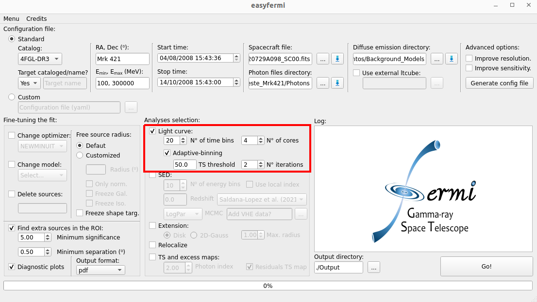
N_Bins: The number of time bins set up in the graphical interface as “N° of time bins”.
Radius: All sources within this radius (centered on the target) are free to vary in the fit. This radius is set as half of the RoI width (see Binned likelihood analysis) or defined by the user within the box “Radius” within the “Fine-tuning the fit” box.
N_cores: Number of cores read from the graphical interface as “N° cores”.

Note

easyfermi will look for preexisting light curves with the same number of time bins set up in the graphical interface. If, for instance, you already produced a light curve with 20 bins, and you are asking for a new light curve with 20 bins, easyfermi will give you a warning in the log, and skip the light curve computation.

Adaptive-binning light curve

This method allows for the computation of a light curve with adaptive time bins, giving us much more information about the variability of the target. It requires a precomputed light curve with constant time bins, as show in the section Constant time bins.

Here we do a loop over every bin of the precomputed light curve and check if the TS of that bin is larger than \(2~\times~ TS_{Threshold}\), where \(TS_{Threshold}\) is read from the graphical interface as “TS threshold”. For the bins at which this condition is satisfied, we apply the fermipy function lightcurve() again with:

N_Bins = int(  (TS of the current bin)/(TS_{Threshold})  )

Such that N_Bins is the lower closest integer to this ratio. For a target with a relatively constant gamma-ray emission, the new bins will all have \(TS \sim TS_{Threshold}\).

For each new run of lightcurve() for a specific bin, we adopt the local data files (i.e. ft1_00.fits, srcmap_00.fits, bexpmap_00 etc) produced by fermipy.

The parameter N_iter is read from the graphical interface as “N° iterations” and tells easyfermi how many times it should rerun the function lightcurve() in the latest light curve available. For instance, if N_iter = 2 and there is no precomputed light curve, easyfermi will first run the constant-binning light curve (see Constant time bins), then compute an adaptive-binning light curve by increasing the time resolution of the bins with \(TS > 2 ~\times~ TS_{Threshold}\), and then compute a third (even finer) adaptive-binning light curve by increasing the resolution of the remaining bins with \(TS > 2 ~\times~ TS_{Threshold}\). In summary: the higher is the value of N_iter, the higher is the final resolution of the light curve.

This method of computing an adaptive-binning light curve is different from the method described in Lott et al. 2012, and presents some advantages and disadvantages:

Pros:

Analysis can be done in parallel (except for Mac OS).
Analysis becomes faster and faster at each new iteration, since we select only the bins that satisfy \(TS > 2 \times TS_{Threshold}\).

Cons:

We can eventually run into upper limits, especially if we set \(TS_{Threshold} < 50\).

Note

We recommend setting \(TS_{Threshold} \geq 50\). With smaller threshold values we can achieve higher time resolution, however, we increase the probability of running into upper limits.

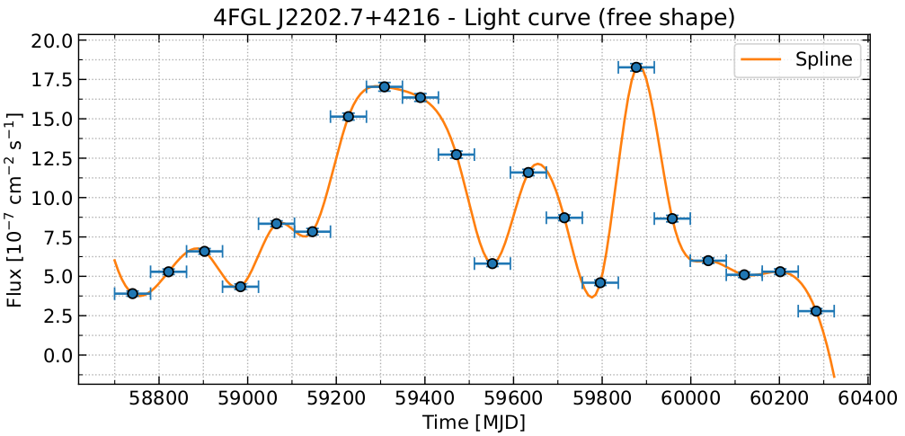
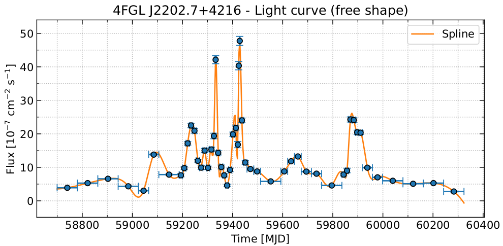
In the figures below, we show the constant- and adaptive-binned light curves for BL Lac from 04/08/2019 15:43:36 up to 14/01/2024 15:43:00 and in the energy range 100 MeV up to 300000 MeV, during some major flaring activity. Since in this especific case we have extraordinary statistics, we set \(TS_{Threshold} = 5000\) and 2 iterations for the adaptive-binned light curve. We see that both light curves present the same overall behavior, although in the adaptive-binned case we can recover much more information (in this specific case, the statistics is so high that we barely can see the error bars).