Spectral energy distribution (SED)
Standard SED
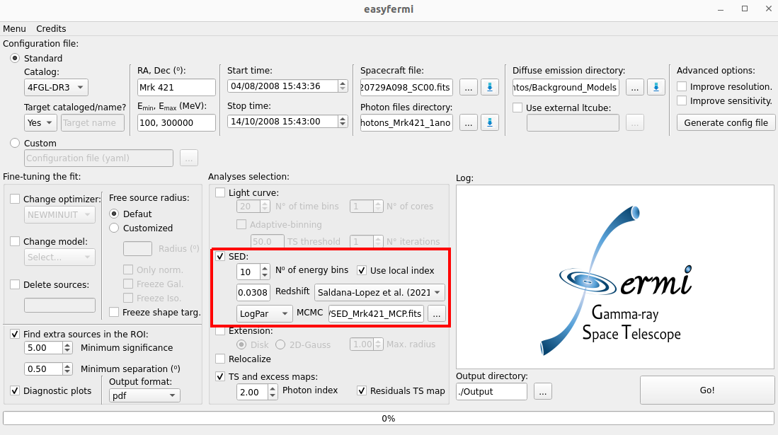
The standard SED generated with easyfermi uses the fermipy function sed() with the following configuration:
sed(Target_Name,loge_bins=N_energy_bins,make_plots=False,use_local_index=use_local_index,write_npy=False)
Where the input parameters are:
Target_Name: This is the name of the target as listed in the adopted Fermi-LAT catalog or the target name written in the field “Target name” in the graphical interface.
N_energy_bins: The number of energy bins set up in the graphical interface as “N° of energy bins”.
use_local_index: If the box Use local index is checked in the graphical interface, we use a power-law approximation to the shape of the global spectrum in each bin. If not checked, then a constant index, \(\gamma = 2\), will be adopted for all energy bins.
The parameters make_plots and write_npy are always set as False in easyfermi. For more details on them, see the fermipy sed documentation.
Extragalactic background light (EBL) absorption correction
This method corrects the EBL absorption observed in the highest energy bins in the SEDs of extragalactic targets using the gammapy class EBLAbsorptionNormSpectralModel. This correction will be applied to any analysis as long as the box Redshift has a value above zero. The user can then select which EBL absorption model to use, where the options are:
If this correction is applied, the MCMC estimation (see Section MCMC) of parameters will be performed in the corrected SED.
Markov Chain Monte Carlo (MCMC)
The estimation of parameters with MCMC in easyfermi is done with emcee and it requires a minimum number of 3 data points with \(TS > 9\). The likelihood function that we maximize in easyfermi is given by:
\(\mathcal{L} = - \frac{1}{2}\sum_n\left[ \frac{(y_n - f(\vec\theta,x_n))^2}{\sigma_n^2} \right]\)
where the sum is performed over all data points with \(TS > 9\), \(y_n\) and \(x_n\) are the y (differential flux) and x (energy) values for each data point, \(\sigma_n\) is the error associated with the \(y\) component of each data point, and \(f(\vec\theta,x_n)\) is the adopted specral model feeded with a set of parameters \(\vec\theta\).
The spectral models available for the MCMC are:
PowerLaw: \(\frac{dN}{dE} = N_0\left(\frac{E}{E_0} \right)^{-\alpha}\), i.e the classical power-law function, where \(\frac{dN}{dE}\) is in units of \(\mathrm{cm}^{-2}\mathrm{s}^{-1}\mathrm{MeV}^{-1}\), \(E\) is in MeV, and the priors are -15 < \(\log(N_0)\) < -8 and 0.5 < \(\alpha\) < 5.0.
LogPar: \(\frac{dN}{dE} = N_0\left(\frac{E}{E_0} \right)^{-\alpha -\beta\log(E/E_0)}\), i.e. the classical log-parabola function, where \(\frac{dN}{dE}\) is in units of \(\mathrm{cm}^{-2}\mathrm{s}^{-1}\mathrm{MeV}^{-1}\), \(E\) is in MeV, and the priors are set to -15 < \(\log(N_0)\) < -8, 1.0 < \(\alpha\) < 4.0, and -1 < \(\beta\) < 1.0.
LogPar_MTT: \(S(E) = S_p10^{-\alpha\log^2_{10}(E/E_p)}\), which is another parametrization of the log-parabola, conveniently giving us the differential energy flux at the log-parabola peak, \(S_p\) [MeV \(\mathrm{cm}^{-2}\mathrm{s}^{-1}\)], the position of this peak in the energy axis, \(E_p\) [MeV], and the spectral curvature \(\alpha\). The priors are set to -7 < \(\log(S_p)\) < -1, -1.0 < \(\alpha\) < 1.0, and 2 < \(E_p\) < 7. The suffix “MTT” stands for Massaro et al. (2004), Tanihata et al. (2004), and Tramacere et al. (2007), which are the first works reporting this parametrization of the log-parabola curve.
PLEC: \(\frac{dN}{dE} = N_0\left(\frac{E}{E_0} \right)^{-\alpha} e^{-(E/E_0)^b}\), i.e. a power-law with a super exponential cutoff, where \(\frac{dN}{dE}\) is in units of \(\mathrm{cm}^{-2}\mathrm{s}^{-1}\mathrm{MeV}^{-1}\) and \(E\) is in MeV. The priors are set to -15 < \(\log(N_0)\) < -8, 1.0 < \(\alpha\) < 4.0, 3.0 < \(E_c\) < 7.0, and 0.2 < \(b\) < 3.0.
PLEC_bfix: same as above, but with \(b \equiv 1\).
PLEC_deMenezes: \(S(E) = S_p\left(\frac{E_p}{E} \right)^{\alpha-2} e^{((2-\alpha)/b)(1-(E/E_p)^b)}\), which is a parametrization of the PLEC developed for
easyfermiconveniently giving us the differential energy flux at the PLEC peak, \(S_p\) [MeV \(\mathrm{cm}^{-2}\mathrm{s}^{-1}\)], the position of this peak in the energy axis, \(E_p\) [MeV], the power law spectral index \(\alpha\), and the super-exponential index \(b\). With this model one can directly estimate \(S_p\), \(E_p\), and their corresponding errors without recurring to huge error propagation formulas. If you use this parametrization in another context, please cite theeasyfermipaper de Menezes (2022) and this documentation. The priors are set to -8 < \(\log(S_p)\) < -1, 0 < \(\alpha\) < 4.0, 2.0 < \(E_p\) < 7.0, and 0.01 < \(b\) < 3.0.
Finally, we adopt 300 walkers, iterate them 500 times, and fix \(E_0 \equiv E_{min}\), where \(E_{min}\) is read from the graphical interface or from the customized configuration file.
Note
The upper limits (i.e. any energy bin with TS < 9) are not included in the MCMC parameter estimation.
VHE table format
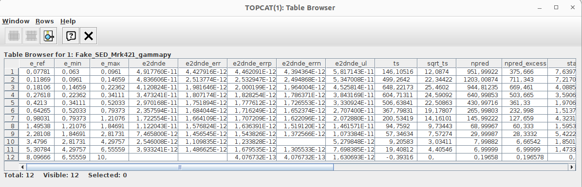
The format of the VHE data table is a standard SED table produced with gammapy 1.1.
It will work with any .fits table, as long as this table contains the following columns in the first extension HDU (e.g. hdul[1].data):
e_ref, e_min, and e_max, all in TeV
e2dnde, e2dnde_err, e2dnde_ul, all in TeV cm-2 s-1
ts
In the figure below we show you how this table should look like (this is actually fake data for Mrk 421).
Model selection with the Akaike information criterion
As a tool for model selection, easyfermi provides the Akaike information criterion (AIC). The AIC is printed in the easyfermi log and saved in the files Target_results.txt and TARGET_NAME_sed.fits.
We use a slightly modified form of this method defined as:
\(AIC = 2k + 2ln(-\mathcal{L}_{max})\),
where k is the number of free parameters in the given model, and \(\mathcal{L}_{max}\) is the maximized likelihood function defined above.
Given a set of candidate models for the data, the preferred model is the one with the minimum AIC value. For the same dataset, two spectral models can be compared by the following expression:
\(e^{(AIC_{min} − AIC_{test})/2}\).
For instance, let’s suppose that you have the spectral data for Mrk 421 and you try to fit this data with a power law (PL) and then with a log-parabola (LP). Let’s also suppose that \(AIC_{PL} = 6.1\) and \(AIC_{LP} = 7.5\). Since the minimum AIC is achieved for the PL model, this means that the LP model is
\(e^{(6.1 − 8.5)/2} = 0.301\) times as probable as the power-law model to minimize the information loss.
Data points with less than 5 photons
The likelihood ratio method adopted in the fermitools, fermipy and easyfermi attributes higher significance to higher energy photons, such that a couple of photons with energies > 100 GeV can easily reach TS > 25. For source detection, this is perfectly fine, since the background at these energies is relatively low and the photon/hadron separation and direction reconstructed by LAT are much better than at low energies (e.g. below 1 GeV). This means that if you detect 2 photons with more than 100 GeV coming from the same position in the sky, it is indeed very likely that there is a gamma-ray source there.
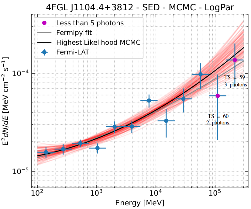
There is, however, a subtle but important difference between being able to detect a source and being able to measure its flux. When trying to build an SED, for instance, the highest-energy bins may have only a few photons and still give you relatively high TSs. In the figure below, we show the spectrum of Mrk 421 observed over 2 months. We see that the highest-energy bins have TSs ~ 60, although we have only 2 or 3 photons for each bin. The differential flux measurements with such a low number of photons is prone to strong fluctuations that can possibly affect the modeling of the SED. Furthermore, we cannot trust statistical error bars if the measurement is not done in a statistically valid sample (i.e. a large number of counts).
In easyfermi, we warn the users about this issue by checking how many photons within a radius of 0.5° from the RoI center are detected for all the SED bins with energies > 10 GeV. If a specific bin has less than 5 photons, it will apear as a magenta point in the SED quickplot. These warnings are saved in the column “Warning_few_photons” in the TARGET_NAME_sed.fits file and can help the users in the task of selecting or not these data points when trying to fit a model.