Basic Analysis
Binned likelihood analysis
The binned likelihood analysis performed in easyfermi starts by instantiating the fermipy class GTAnalysis and feeding it with a configuration file (i.e. ‘config.yaml’) generated with the information given by the user in the graphical interface. The standard event classification and event type are set as evclass=128 and evtype=3, but these values can be changed by the user by checking the box Improve resolution or if the analysis is done in the Custom mode.
The region of interest (RoI) width and zenith angle (\(z_{max}\)) cut adopted in the Standard mode of easyfermi depend on the minimum energy set up in the graphical interface. In summary, if
\(E_{min} < 100\) MeV, the RoI width is set to 17°, and \(z_{max} = 80°\).
\(100 \leq E_{min} < 500\) MeV, the RoI width is set to 15°, and \(z_{max} = 90°\).
\(500 \leq E_{min} < 1000\) MeV, the RoI width is set to 12°, and \(z_{max} = 100°\).
\(E_{min} \geq 1000\) MeV, the RoI width is set to 10°, and \(z_{max} = 105°\).
For all these cases, we also include in the model all the cataloged sources lying in a region 10° larger than the width of the RoI (i.e. we set src_roiwidth : roi_width + 10 in the configuration file). All these values can be changed by the user in the Custom mode of easyfermi. Similarly, the data downloaded directly from the graphical interface contain photons within a region with radius \(14°~\mathrm{if}~E_{min} < 100\) MeV, \(12°~\mathrm{if}~~100 \leq E_{min} < 500\) MeV, \(11°~\mathrm{if}~~500 \leq E_{min} < 1000\) MeV, and \(9°~\mathrm{if}~E_{min} \geq 1000\) MeV. Furthermore, if the box Improve sensitivity is checked, the data will be split into 2 or 3 energy components (depending on \(E_{min}\)) and \(z_{max}\) will then assume the values shown above for each one of these components (if \(E_{min} < 500\) MeV, the lowest energy component will have \(z_{max} = 90°\) if \(E_{min} \geq 100\) MeV, and \(z_{max} = 80°\) otherwise).
The remaining Standard configuration of easyfermi is:
edisp : True, for the energy dispersion.
irfs : ‘P8R3_SOURCE_V3’, for the instrument response function.
edisp_disable : [‘isodiff’], to disable the energy dispersion correction in the isotropic component.
edisp_bins : -2, to add two extra energy bins when accounting for energy dispersion.
All the intermediate analsyis files, such as ccube, ltcube, srcmaps, and exposure map are generated with the fermipy function setup(). Once the setup is done, easyfermi computes a counts map (saved in the output directory as cmap.fits) by summing all the energy components of the ccube.fits file.
Note
For analyses in a time window larger than 1 year, the computation of the ltcube can take several hours to finish. In extreme situations, e.g. if you ara analyzing 14 years of data and check the box “improve sensitivity” on the graphical interface, the computation of the ltcube can take more than 20 hours.
If you want to analyze different targets in the same time window and energy interval, you don’t need to compute the ltcube multiple times. You compute it once, and for the subsequent analyses you can simply import the ltcube list file (called “ltcube_list.txt” and saved in the output directory) under the checkbox “Use external ltcube”.
The next step in the analysis is calling the fermipy function optimize() with the following configuration:
optimize(npred_frac=0.95, npred_threshold=50, shape_ts_threshold=30)
This function optimizes the RoI model in three sequential steps:
Free the normalization of the N largest components (as determined from NPred) that contain a fraction npred_frac of the total predicted counts in the model and perform a simultaneous fit of the normalization parameters of these components.
Individually fit the normalizations of all sources that were not included in the first step in order of their Npred values. Skip any sources that have NPred < npred_threshold.
Individually fit the shape and normalization parameters of all sources with TS > shape_ts_threshold where TS is determined from the first two steps of the ROI optimization.
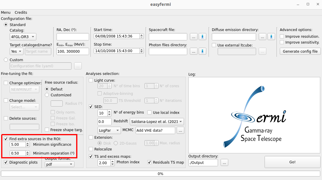
After the optimization, we give the option to the user to call the fermipy function find_sources() (by checking the box Find extra sources in the ROI, as shown in the figure below) with the following configuration:
find_sources(sqrt_ts_threshold=Minimum_significance, min_separation=Minimum_separation, multithread=True)
which will look for possible non-cataloged gamma-ray sources by generating a TS map for the RoI and identify peaks with \(\sqrt{TS} >\) Minimum_significance and an angular separation of at least Minimum_separation from a higher amplitude peak in the TS map. This method can run several times until no sources with \(sqrt(TS) >\) Minimum_significance are found. The values for Minimum_significance and Minimum_separation can be defined by the user in the graphical interface.
The standard fit in easyfermi is done with the fermipy function fit() with NewMinuit as the optimizer, although this can be changed by the user in the checkbox Change optimizer. The radius within which the parameters of all sources are free to vary (normalization and spectral shape) is set as half the RoI width (see the second paragraph of this section), but can be changed by the user in the panel Free source radius, under the Customized button. The adopted spectral model for the target will be that listed in the selected Fermi-LAT catalog (default is 4FGL-DR3) or a power law if the target is not listed in the selected catalog. This model can be changed at any time by the user under the box Change model, and the complete description of all available models can be found here.
If the fit does not converge, easyfermi:
deletes all sources with \(TS < TS_{cut}\) from the RoI or…
deletes all sources with \(TS < TS_{target}\) if \(TS_{target} < TS_{cut}\).
reruns the fit.
The default value for \(TS_{cut}\) is 16, but the user can change this value in panel Fine-tuning the fit in the graphical interface.
If even after that the fit does not converge, the user can freely modify the parameters in the panel Fine-tuning the fit and rerun the analysis.
Note
The \(TS_{target}\) threshold was fixed at 25 until easyfermi 2.0.7.
Once the RoI fit is done, the results are saved in the output directory in the file Target_results.txt (for a quick look at the target parameters) and in the file Results.fits (for all sources in the RoI).
Non-cataloged target
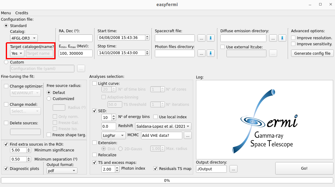
If your target is not listed in the adopted Fermi-LAT catalog, you have to set the combo box Target cataloged/name to No (see figure below) and give a nickname to your target. It can be any name you want. This target will be added as a point-source with a power-law spectrum, but you can change this spectral model under the box Change model.
Diagnostic plots
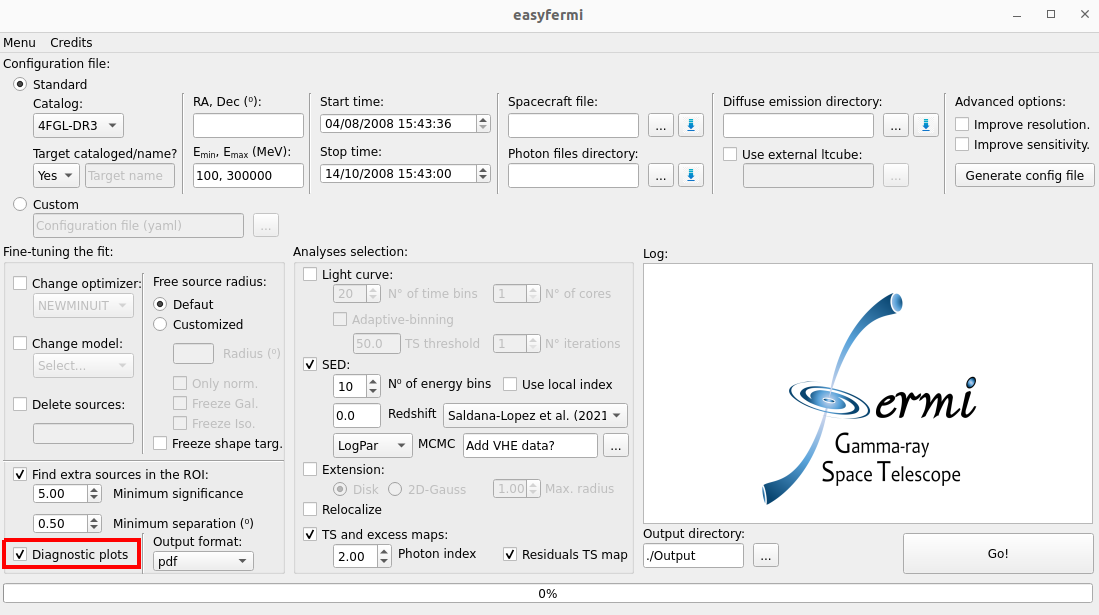
If the box Diagnostic plots is checked (see figure below), all of the diagnostic plots created by fermipy are saved in the output directory, such as the model map, the excess map, the y and x counts profile, etc.
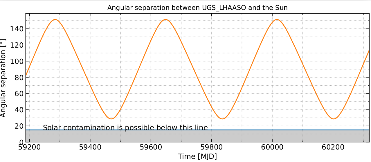
The novelty diagnostic plot of easyfermi is the angular separation between the target and the Sun within the given time window. We compute this separation based on the data available in the Fermi-LAT spacecraft file and using the astropy class SkyCoord(). This plot is useful, e.g., to look for possible solar contamination on your SED or light curve. In the figure below, we show the diagnostic plot for the angular separation between the target 1LHAASO J1219+2915 and the Sun over the period of ~3 years.