Custom analysis

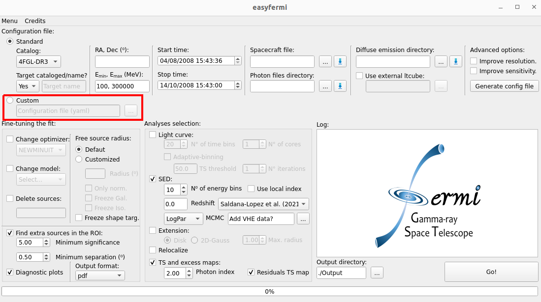
Here we give you some examples on how to customize your analysis with easyfermi. In summary, you simply have to modify a configuration file and upload it in the easyfermi window as indicated in the figure above.

If you don’t know where to start with your own configuration file, you can add the coordinates (or name), desired energy and time ranges, and the paths to the data files under the “Standard” button in the easyfermi main window and then click in the button “Generate config file”. This action will generate a ‘config.yaml’ file within the output directory, allowing you full flexibility to customize it according to your preferences.

Note

If you check the boxes “Improve resolution” and/or “Improve sensitivity”, the config.yaml file generated with the button “Generate config file” will be modified accordingly.

Below we give you some examples of customized configuration files.

Precise selection of time intervals

Tutorial available on YouTube.

Let’s suppose you want to build the average SED for 3 specific time windows for BL Lac. In this case, the only feature you need to add to the “config.yaml” file is the line “filter”, as indicated in the highlighted line below.

data:
  evfile : /home/user/Documentos/GUI/Tutorials/BLLac/Output/list.txt
  scfile : /home/user/Documentos/spacecraft/L240206050150320729A098_SC00.fits

binning:
  roiwidth   : 15
  binsz      : 0.1
  binsperdec : 8

selection :
  emin : 100.0
  emax : 300000.0
  zmax    : 90
  evclass : 128
  evtype  : 3
  ra: 330.68038041666665
  dec: 42.277771944444446
  tmin: 638496005
  tmax: 655776005
  filter: '((START>6.40997722E8) && (STOP<6.41582362E8)) || ((START>6.4909916E8) && (STOP<6.4943324E8))  || ((START>6.4943324E8) && (STOP<6.4976732E8))'

gtlike:
  edisp : True
  irfs : 'P8R3_SOURCE_V3'
  edisp_disable : ['isodiff']
  edisp_bins : -2

model:
  src_roiwidth : 25
  galdiff  : '/home/user/Documentos/Background_Models/gll_iem_v07.fits'
  isodiff  : '/home/user/Documentos/Background_Models/iso_P8R3_SOURCE_V3_v1.txt'
  catalogs : ['4FGL-DR3']

Customized resolution and better SED for a target on the Galactic plane

At the cost of decreasing the sensitivity, you can cut the photons with worst positional reconstruction from your dataset by selecting only the photons lying within the best PSF quartiles (details here.)

Below we give the example of a config.yaml file generated with the button “Generate config file” for Mrk 501, and then we discuss how you can modify it to analyze the data that better suits your goals.

This config.yaml file was generated with the boxes “Improve resolution” and “Improve sensitivity” checked. Checking the box “Improve sensitivity” for such a large energy range (i.e. from 100 MeV up to 800 GeV), means that we will perform the Fermi-LAT analysis for three different energy components, tuned to improve sensitivity at the highest energies (see Basic Analysis).

Note

Even if you are not interested in a better resolution, you can use this method to improve the quality of your low energy (i.e. < 500 MeV) SED data points. For instance, if your target is in the Galactic plane, where the contamination levels are very high at low energies, a standard analysis eventually gives you an SED where the lowest energy data points seem too high to be true (e.g. more than \(3\sigma\) away from the fitted model). This happens because several badly reconstructed photons that do not belong to your target are being swallowed into your analysis. So if you are analyzing a strong source in the Galactic plane, it is typically a good idea to remove the low-energy photons with the worst reconstruction (i.e. PSF0) from your analysis.

data:
  evfile : /home/user/Documentos/GUI/easyFermi/code/LHAASO_counterparts/Output_Mrk501/list.txt
  scfile : /home/user/Documentos/GUI/easyFermi/code/LHAASO_counterparts/spacecraft/L240204110942320729A088_SC00.fits

binning:
  roiwidth   : 15
  binsz      : 0.1
  binsperdec : 8

selection :
  emin : 100.0
  emax : 800000.0
  zmax    : 90
  evclass : 128
  evtype  : 48
  ra: 253.46756916666664
  dec: 39.76016888888889
  tmin: 636249601
  tmax: 686275200

gtlike:
  edisp : True
  irfs : 'P8R3_SOURCE_V3'
  edisp_disable : ['isodiff']
  edisp_bins : -2

model:
  src_roiwidth : 25
  galdiff  : '/home/user/Documentos/Background_Models/gll_iem_v07.fits'
  isodiff  : '/home/user/Documentos/Background_Models/iso_P8R3_SOURCE_V3_v1.txt'
  catalogs : ['4FGL-DR3']

components:
  - model:
      galdiff  : '/home/user/Documentos/Background_Models/gll_iem_v07.fits'
      isodiff  : '/home/user/Documentos/Background_Models/iso_P8R3_SOURCE_V3_v1.txt'
    selection:
      emin : 100.0
      emax : 500
      zmax : 90
      evtype : 48
  - model:
      galdiff  : '/home/user/Documentos/Background_Models/gll_iem_v07.fits'
      isodiff  : '/home/user/Documentos/Background_Models/iso_P8R3_SOURCE_V3_v1.txt'
    selection:
      emin : 500
      emax : 1000
      zmax : 100
      evtype : 56
  - model:
      galdiff  : '/home/user/Documentos/Background_Models/gll_iem_v07.fits'
      isodiff  : '/home/user/Documentos/Background_Models/iso_P8R3_SOURCE_V3_v1.txt'
    selection:
      emin : 1000
      emax : 300000.0
      zmax : 105
      evtype : 3

We see that for the lowest-energy component (i.e. 100 MeV up to 500 MeV), we use only PSF 2 and 3 events (i.e. evtype = 48), equivalent to 50% of all photons detected in this energy range, while in the medium energy range (i.e. from 500 MeV up to 1 GeV), we use PSF 1, 2 and 3 (evtype = 56), equivalent to 75% of all photons detected in this energy band. So let’s suppose you prefer to include all photons with more than 500 MeV in your analysis (i.e. evtype : 3). The only thing you need to do is to modify the highlighted line in the following part of the file:

[...]
- model:
      galdiff  : '/home/user/Documentos/Background_Models/gll_iem_v07.fits'
      isodiff  : '/home/user/Documentos/Background_Models/iso_P8R3_SOURCE_V3_v1.txt'
    selection:
      emin : 500
      emax : 1000
      zmax : 100
      evtype : 3
[...]

But how do you know which evtype number to choose for different PSF selections? The detailed answer is provided here.

You can also play with the zenith angle cut. The recommended zenith angle cuts (zmax in the config.yaml file) selections have been optimized to reduce the limb contamination to a negligible level (< 5% of the total diffuse emission at high latitudes). For diffuse analysis more restrictive selections may be required. For evtype = 3, the recommended zenith angle cuts are:

80°, for \(E_{min} > 50\) MeV
90°, for \(E_{min} > 100\) MeV
95°, for \(E_{min} > 200\) MeV
100°, for \(E_{min} > 300\) MeV
100°, for \(E_{min} > 500\) MeV

For \(E_{min} > 1\) GeV, it is common practice to set zmax = 105, but try avoiding zenith angle cuts larger than that.

Customized extended emission

easyfermi provides the users with two simple spatial models for extended emission, which are a disk and a 2D Gaussian. If you want to do your own spatial model, please see Extension - Advanced.

Adjusting the parameter ranges of a spectral model

Let’s say you want to modify the values and/or ranges for the parameters in a spectral model before performing the fit. Here are the steps you must follow:

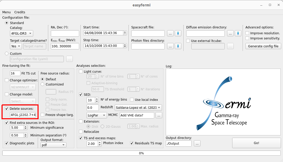
If your target is listed in the adopted FGL catalog, you must delete it from the model using the check-box “Delete sources”. E.g. if your RoI is centered on the source 4FGL J2202.7+4216, you can do as in the figure below:

_images/easyfermi_window_delete_source.png

Now manually add your target to the config.yaml file setting the parameter values and ranges as you prefer. This name cannot contain blank spaces as e.g. “NGC 1022”, neither it can be listed in the adopted Fermi-LAT catalog, as e.g. “Mkn_421”, so please give it single name not listed in the LAT catalog, like “SourceA”, “NGC_1022”, “Super_duper_Mkn_421”, or something else in this line. In the figure below we show the example for a power-law model:

data:
  evfile : /home/user/Documentos/GUI/Tutorials/BLLac/Output/list.txt
  scfile : /home/user/Documentos/spacecraft/L240206050150320729A098_SC00.fits

binning:
  roiwidth   : 15
  binsz      : 0.1
  binsperdec : 8

selection :
  emin : 100.0
  emax : 300000.0
  zmax    : 90
  evclass : 128
  evtype  : 3
  ra: 330.68038041666665
  dec: 42.277771944444446
  tmin: 638496005
  tmax: 655776005
  filter: '((START>6.40997722E8) && (STOP<6.41582362E8)) || ((START>6.4909916E8) && (STOP<6.4943324E8))  || ((START>6.4943324E8) && (STOP<6.4976732E8))'

gtlike:
  edisp : True
  irfs : 'P8R3_SOURCE_V3'
  edisp_disable : ['isodiff']
  edisp_bins : -2

model:
  src_roiwidth : 25
  galdiff  : '/home/user/Documentos/Background_Models/gll_iem_v07.fits'
  isodiff  : '/home/user/Documentos/Background_Models/iso_P8R3_SOURCE_V3_v1.txt'
  catalogs : ['4FGL-DR3']
  sources  :
    - { name: 'SourceA', ra : 330.68038, dec : 42.27777,
     SpectrumType : 'PowerLaw',
     Prefactor : {value: 1.0, scale : !!float 1e-11, free : "1", max : "1000", min : "1e-03"},
     Index : {value: 2.0, scale : "-1", free : "1", max : "3", min : "1.5"},
     SpatialModel: 'PointSource' }

If instead of a power-law you are interested in a log-parabola or PLEC (equivalent to PLSuperExpCutoff in the LAT spectral models), you can change the last part of the configuration file to:

[...]

model:
  src_roiwidth : 25
  galdiff  : '/home/user/Documentos/Background_Models/gll_iem_v07.fits'
  isodiff  : '/home/user/Documentos/Background_Models/iso_P8R3_SOURCE_V3_v1.txt'
  catalogs : ['4FGL-DR3']
  sources  :
    - { name: 'SourceA', ra : 330.68038, dec : 42.27777,
     SpectrumType : 'LogParabola',
     norm : {value: 1.0, scale : !!float 1e-11, free : "1", max : "1000", min : "1e-03"},
     alpha : {value: 2.0, scale : "1", free : "1", max : "3", min : "1.5"},
     beta : {value: 0.1, scale : "1", free : "1", max : "1", min : "0"},
     SpatialModel: 'PointSource' }

or

[...]

model:
  src_roiwidth : 25
  galdiff  : '/home/user/Documentos/Background_Models/gll_iem_v07.fits'
  isodiff  : '/home/user/Documentos/Background_Models/iso_P8R3_SOURCE_V3_v1.txt'
  catalogs : ['4FGL-DR3']
  sources  :
    - { name: 'SourceA', ra : 330.68038, dec : 42.27777,
     SpectrumType : 'PLSuperExpCutoff',
     Prefactor : {value: 1.0, scale : !!float 1e-11, free : "1", max : "1000", min : "1e-03"},
     Index1 : {value: 2.0, scale : "1", free : "1", max : "3", min : "1.5"},
     Cutoff : {value: 1, scale : "1e+04", free : "1", max : "100", min : "0.01"},
     Index2 : {value: 0.1, scale : "1", free : "1", max : "4", min : "0"},
     SpatialModel: 'PointSource' }

For other spectral models you can follow the exact nomenclature of parameters found in the LAT Source Model Definitions. The equiavalencies between easyfermi and Fermitools spectral models are ‘Power-law’: ‘PowerLaw’, ‘Power-law2’: ‘PowerLaw2’, ‘LogPar’: ‘LogParabola’, ‘PLEC’: ‘PLSuperExpCutoff’, ‘PLEC2’: ‘PLSuperExpCutoff2’, ‘PLEC3’: ‘PLSuperExpCutoff3’, ‘PLEC4’: ‘PLSuperExpCutoff4’, ‘BPL’: ‘BrokenPowerLaw’, ‘ExpCutOff-EBL’: ‘ExpCutoff’.
Now upload your modified configuration file under the button “Custom” and press “Go!”. That’s all.